"Demystifying Naïve Bayes: Log Probability and Laplace Smoothing"

Before moving forward pls read this article first then you can understand further ….

Agenda:

Advancing Naive Bayes

. Types of Naive Bayes

1. The Concept of Log Probability
2. The Concept of Laplace Smoothing

Numerical stability 

In the earliest days of programming, developers often encountered difficulties when it came to storing decimal or floating-point values in computer memory. While they could easily represent whole numbers, representing decimal values posed a challenge.

The reason behind this challenge is that computers use binary representation, using only 0s and 1s, to represent any number. Consequently, it becomes challenging to accurately represent decimal values in binary form. For instance, when representing extremely small numbers like 0.000001, precision can be lost, and the value may be treated as 0.

Let's consider an example in the field of biology. Suppose you are measuring the radius of a cell. In some cases, your measurements might be extremely small, such as 0.00000001. Now, let's say you want to compare this radius to another cell's radius, which is 0.0000003. Due to the limitations of computer representation, the computer will treat both values as zero, leading to the incorrect conclusion that both cells have equal radii. This condition is referred to as underflow.

Underflow refers to a situation in which values smaller than the smallest representable value in a computer's numeric system are rounded down to zero.

Let's explore underflow in the context of a simple example. Suppose you are trying to predict whether a student will get a placement based on their CGPA (Cumulative Grade Point Average) and IQ (Intelligence Quotient). Let's say the student has a CGPA of 8.1 and an IQ of 81. To calculate the probability of placement, you need to evaluate the following:

p(y|8.1, 81) = p(y) * p(8.1|y) * p(81|y) 

p(n|8.1, 81) = p(n) * p(8.1|n) * p(81|n)

Since probabilities range from 0 to 1, when you multiply these probabilities together (especially if you have multiple features), the result tends to move closer to zero. This leads to the underflow problem, where the computed probability becomes extremely small, approaching zero, and can cause inaccuracies in the prediction model.

To address the underflow problem, one solution is to work with

logarithmic probabilities

 logarithmic probabilities. By taking the logarithm of the probabilities, you can avoid the issue of extremely small values.

The logarithmic property you mentioned, log(A * B) = log(A) + log(B), is indeed a useful property. It allows us to rewrite the expression.

 log(p(y) * p(8.1|y) * p(81|y)) as the sum of logarithms: 

log(p(y)) + log(p(8.1|y)) + log(p(81|y)).

In the context of implementing this solution, you can utilize the predict_log_proba(X) function available in the scikit-learn library's Naive Bayes implementation. This function computes the logarithm of the probabilities for each class given input features X.

After calculating the logarithmic probabilities, you can compare them and choose the class with the highest log probability. For example, if you obtain a log probability of 53 for one class and 25 for another, you would select the class with the higher log probability.

By using logarithmic probabilities, you can overcome the underflow problem and make more accurate predictions.

Laplace additive smoothing

To understand why we need Laplace additive smoothing, 

let's consider a sentiment analysis task. We have two features: movie reviews and corresponding sentiments (positive or negative). 

Our goal is to predict the sentiment based on the movie review.

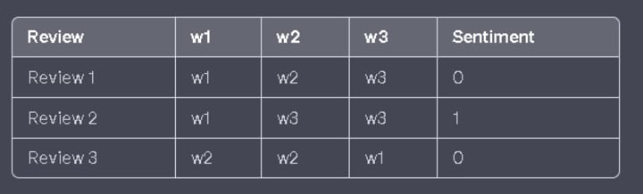
To convert this data into a binary bag-of-words table, we need to represent each word with a binary value (0 or 1).

 The table would look like this:

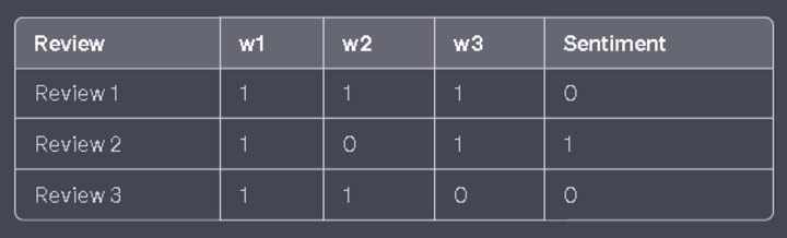
In the binary bag-of-words table, each word corresponds to a column, and its presence is denoted by a 1, while its absence is denoted by a 0. The sentiment is represented by the "Sentiment" column.

To create the binary bag-of-words representation table, considering the additional query point "r4" with the words "w1, w1, w1," we can convert it to a table as follows

:

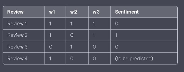
In this table, "r4" represents the additional query point, where "w1" appears twice and "w2" and "w3" are absent. The sentiment for Review 4 is yet to be predicted.

Now, let's calculate the probabilities for positive and negative sentiments based on the given data table:

p(+ve|r4) = p(+ve) * p(w1=1|+ve) * p(w2=0|+ve) * p(w3=0|+ve) = (2/3) * (1/1) * (1/1) * (0/1) = 0

p(-ve|r4) = p(-ve) * p(w1=1|-ve) * p(w2=0|-ve) * p(w3=0|-ve) = (1/3) * (1/2) * (0/2) * (1/2) = 1/12

As you can see, both probabilities become 0, which is an issue when certain features do not exist in a particular class, resulting in zero probabilities. This is where Laplace additive smoothing comes in.

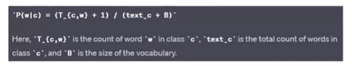
Laplace additive smoothing helps avoid zero probabilities by adding a small constant (alpha) to the numerator and n * alpha to the denominator of each probability estimate. By applying Laplace additive smoothing, the probabilities will never be zero.

The value of alpha is usually 1 (default), but you can choose a different value based on your preference. The value of n depends on the type of Naive Bayes algorithm you are using, which we can discuss further if needed.

Let's understand the bias-variance tradeoff in the case of Naive Bayes.

 The question arises: why do we add alpha in the numerator and n * alpha in the denominator? 

Why don't we add a very small constant value like 0.000001 instead?

The reason we add alpha in the numerator and n * alpha in the denominator is to have flexibility in controlling the bias and variance of the model. By tuning the value of alpha, we can adjust the bias and variance accordingly.

When a model has high bias, it means it has simplified assumptions or constraints that may lead to underfitting, resulting in poor performance. In such cases, we can set a lower value of alpha to reduce bias and allow the model to capture more complex patterns.

On the other hand, when a model has high variance, it means it is too sensitive to the training data and may overfit, resulting in poor generalization to unseen data. To address high variance, we can set a higher value of alpha to smoothen the probability estimates and reduce the impact of individual features, thus reducing variance.

Alpha serves as a hyperparameter that allows us to strike a balance between bias and variance. By choosing different values of alpha, we can fine-tune the model's behavior and find the optimal tradeoff between bias and variance for a specific problem.

There are two reasons why we use Laplace additive smoothing:

1. To ensure that probabilities will not become zero.
2. By tuning the value of alpha and n * alpha, we can reduce overfitting and strike a balance between bias and variance trade-off.

Types of Naive Bayes

Let's discuss the five types of Naive Bayes classifiers:

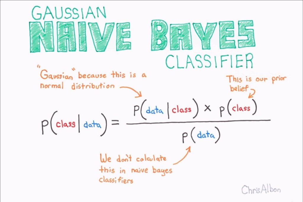
1. Gaussian Naive Bayes: This type of Naive Bayes is used when the dataset consists of numerical features. It assumes that the features follow a Gaussian (normal) distribution. Gaussian Naive Bayes is suitable for continuous data.
2. Categorical Naive Bayes: When the dataset contains categorical features, such as colors or types of objects, we use Categorical Naive Bayes. It assumes that each feature follows a categorical distribution.
3. Bernoulli Naive Bayes: Bernoulli Naive Bayes is applied when the features are binary or follow a Bernoulli distribution. This type of Naive Bayes is suitable for datasets with binary features like presence or absence of certain attributes.
4. Multinomial Naive Bayes: Multinomial Naive Bayes is commonly used for text classification tasks. It assumes that features represent the frequencies or occurrences of different words in the text. It is suitable for datasets with discrete features and follows a multinomial distribution.
5. Complement Naive Bayes: Complement Naive Bayes is a variation of Naive Bayes that is designed to address imbalanced datasets. It is particularly useful when the majority class overwhelms the minority class in the dataset. It aims to correct the imbalance by considering the complement of each class when making predictions.

Each type of Naive Bayes classifier is suitable for different types of datasets based on the nature of the features and their distribution. By selecting the appropriate Naive Bayes algorithm, we can effectively model and classify data based on the given features.

let start with

 Gaussian Naive Bayes

when to use naive bayes which form of dataset 

Data → when we have data like where all the features are numerical at that time, we use gaussian naive bayes.

Let's say we have a dataset containing age and marital status information, where we want to predict whether a person is married or not. For example, we have 5 data points in the dataset.

Now, let's consider a scenario where we want to calculate the probability of a person being married at the age of 55. We predict "yes" for married and "no" for not married. So, we want to calculate

P(yes|55) = (P(55|yes) * P(yes)) / P(w)

P(no|55) =(P(55|no) * P(no)) / P(w)

However, what if we don't have any data points with an age of 55 in our dataset? In that case, both probabilities will be zero because we won't be able to calculate the probability of P(55/yes) or P(55/no).

To handle numerical data in Naive Bayes, we use a different approach. We assume that the particular age column follows a normal distribution (Gaussian distribution) and calculate the mean (μ) and standard deviation (σ) of the age column.

Now, we can assume that the age values follow a Gaussian distribution. We use the formula

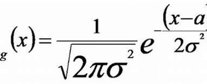
f(x) = 1 / (σ * √(2π)) * e^(-((x - μ)²) / (2 * σ²)).

This formula gives us the probability density.

To calculate the probability, we take the query point (in this case, 55) and plot it on our Gaussian distribution. We calculate the probability density at that point, let's say we get 0.62. This means the probability density to get the age of 55 is 0.62 (not exactly the probability, but the probability density).

It's important to note that for both classes (married and not married), we have two different Gaussian distributions, one for "yes" and another for "no". We calculate the probability density using the respective distribution.

After performing the calculation, we replace P(55/yes) with 0.62. Even though we don't have the exact data point in our dataset, we can calculate the probability using the distribution.

It's worth mentioning that this approach assumes the particular column or feature follows a Gaussian distribution. If the data follows a different distribution, such as a chi-square distribution, we would apply the corresponding formulation for that distribution. If the data doesn't follow any well-known distribution, we would need to explore alternative techniques to handle such cases.

Question on Gaussian NB

why Laplace Additive smoothing does not apply on gaussian Naive Bayes?

Laplace additive smoothing is not applied to Gaussian Naive Bayes because it assumes that the features in the dataset follow a Gaussian (normal) distribution. In Gaussian Naive Bayes, the probability estimation is based on calculating the mean and standard deviation of each feature within each class.

Since Gaussian distributions are continuous, there is no issue of zero probabilities or missing feature values. Laplace smoothing is typically used when dealing with categorical or discrete features, where the presence of zero probabilities can occur when a feature does not appear in a particular class.

Therefore, in the case of Gaussian Naive Bayes, Laplace additive smoothing is not necessary as the Gaussian distribution handles the continuous nature of the features without encountering the problem of zero probabilities.

Categorical Naïve Bayes:

 When the dataset contains categorical features, such as colors or types of objects, we use Categorical Naive Bayes. It assumes that each feature follows a categorical distribution.

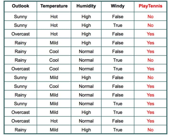
So, over here, what we are going to do is use this simple dataset to understand Naive Bayes. Our goal is to predict whether a student will go to play tennis given these weather conditions.

Let's say we have a query point:

w = {sunny, cool, normal, true}

We need to predict whether the student will go to play tennis (yes or no). We will use Bayes' theorem for this purpose.

The formula is: P(A|B) = (P(B|A) * P(A)) / P(B)

note laplace smoothing is not apply on P(A)

So, our problem formulation is P(yes|w) and P(no|w). Here is the equation:

P(yes|w) = (P(w|yes) * P(yes)) / P(w)

P(no|w) =(P(w|no) * P(no)) / P(w)

By simplifying and removing the denominator from both equations, we can see that they are the same.

The final equation for both probabilities is:

P(yes|w) = (P(w|yes) * P(yes))

note LaPlace smoothing is not apply on P(yes),P(no))

P(no|w) =(P(w|no) * P(no))

P(yes|w) = P(sunny|yes) * P(cool|yes) * P(normal|yes) * P(true|yes) * P(yes) = (2/9) * (3/9) * (6/9) * (3/9) * (9/14)

Applying Laplace smoothing alpha=1,

note LaPlace smoothing is not apply on P(yes)

 n=no.of category present in feature or column

for Outlook (n=3), Temperature (n=3), Humidity(n=2), windy(n=2)

=(2+1/9+3*1) * (3+1/9+3*1) * (6+1/9+2*1) * (3+1/9+2*1) * (9/14)

= 3/12*4/13*7/11*4/11*9/14

=0.01144

(Try calculating it yourself using the given data table.)

P(no|w) = P(sunny|no) * P(cool|no) * P(normal|no) * P(true|no) * P(no)

for more info must read…..

Multinomial Naive Bayes:

Multinomial Naïve Bayes is commonly used for text classification tasks. It assumes that features represent the frequencies or occurrences of different words in the text. It is suitable for datasets with discrete features and follows a multinomial distribution.

Email- spam classification and sentiment analysis are good example

let's we discuss how Multinomial Naive Bayes actually work.

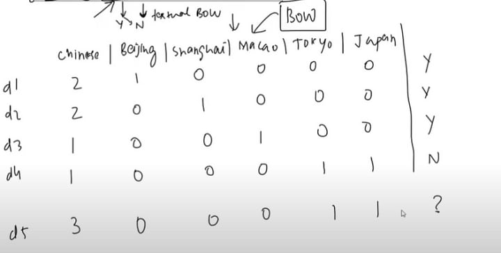
dataset we are going to be use. 

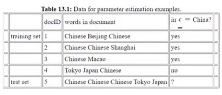
d5 →{Chinese , Chinese, Chinese, Tokyo, Japan}

bag of words →{3,0,0,0,1,1} 

we need to predict whether it is China or not. 

d5 →{Chinese , Chinese, Chinese, Tokyo, Japan}

bag of words →{3,0,0,0,1,1}

P(yes|d5) 

P(Chinese|Yes) * P(Beijing|Yes) * P(Shanghai|Yes) * P(Macao|Yes) * P(Tokyo|Yes) * P(Japan|Yes) * P(Yes)

Now, let's calculate the probabilities 

P(Chinese|Yes) = 5/ 8

P(Beijing|Yes) = 1 / 8

P(Shanghai|Yes) = 1 / 8

P(Macao|Yes) = 1 / 8

P(Tokyo|Yes) = 0 / 8= 0 

P(Japan|Yes) = 0 / 8= 0 

P(Yes) = 3 / 4

After Laplace smoothing, the probabilities for "Tokyo" and "Japan" become non-zero. This is because Laplace smoothing adds a count of alpha=1 in numerator and n*alpha in denominator =6*1

here n is : size of vocabulary of unique words you have

Now, let's calculate the probabilities:

P(Chinese|Yes) = (5 + 1) / (8 + 6) = 6 / 14 = 3 / 7 

P(Beijing|Yes) = (1 + 1) / (8 + 6) = 2 / 14 = 1 / 7

 P(Shanghai|Yes) = (1 + 1) / (8 + 6) = 2 / 14 = 1 / 7 

P(Macao|Yes) = (1 + 1) / (8 + 6) = 2 / 14 = 1 / 7

 P(Tokyo|Yes) = (0 + 1) / (8 + 6) = 1 / 14

 P(Japan|Yes) = (0 + 1) / (8 + 6) = 1 / 14 

P(Yes) = 3/ 4

Now let's recalculate the expression:

d5 →{Chinese , Chinese, Chinese, Tokyo, Japan}

bag of words →{3,0,0,0,1,1}

P(Chinese=3|yes) * P(Beijing=0|yes) * P(shanghai=0|yes) * P(Macao=0|yes) * P(Tokyo=1|yes) * P(Japan=1|yes) * P(yes)

Raising each probability with power, given number of occurrences in d5 like chines occurrence is 3.

P(Chinese|Yes)³ * P(Beijing|Yes)⁰ * P(Shanghai|Yes)⁰ * P(Macao|Yes)⁰ * P(Tokyo|Yes)¹ * P(Japan|Yes)¹ * P(Yes)

= (3/7)³ * (1/7)⁰ * (1/7)⁰ * (1/7)⁰ * (1/14)¹ * (1/14)¹ * (3/4)

Simplifying the expression:

= 27/343 * 1 * 1 * 1 * 1/2744 * 1/2744 * 3/4

= 81/32687648

Therefore, the corrected value of the expression is 81/32687648

Do the same calculation for below:

1. d5 →{Chinese , Chinese, Chinese, Tokyo, Japan}
2. bag of words →{3,0,0,0,1,1}

P(no|d5) =

= P(Chinese=3|no) * P(Beijing=0|no) * P(shanghai=0|no) * P(Macao=0|no) * P(Tokyo=1|no) * P(Japan=1|no) * P(no)

.......

At the end you will find:

P(Yes|d5) > P(No|d5)

d5 -->Chinese, Chinese, Chinese, Tokyo, Japan} - -> Yes

we will discuss. in our Next Post Saty tunned

1. Bernoulli Naive Bayes
2. Complement Naive Bayes:

Also check out our 1st and 3rd post on it

link is given in the comment section.