
"Demystifying Principal Component Analysis: A Comprehensive Guide"
"A Step-by-Step Journey Through Dimensionality Reduction and Data Exploration"

In simple terms, PCA (Principal Component Analysis) is a technique used to simplify and understand complex data. It takes a dataset with many variables and finds the most important patterns or trends in the data.
Imagine you have a large dataset with many different measurements, such as the height, weight, age, income, and education level of people. It can be difficult to make sense of all these variables at once. PCA helps by finding new variables, called principal components, that combine the original variables in a way that captures the most important information.
PCA works by looking for directions in the data along which the variation is the highest. These directions are the principal components. The first principal component explains the largest amount of variation in the data, the second principal component explains the second largest amount, and so on.
By using PCA, you can reduce the complexity of the dataset and focus on the most important aspects. It allows you to understand which variables are most influential and which ones can be safely ignored without losing too much information. Additionally, PCA can help with data visualization by representing the data in a lower-dimensional space, making it easier to see patterns and relationships.
In summary, PCA is a technique that simplifies complex data by finding the most important patterns and reducing the number of variables. It helps to identify the key factors driving the data and allows for easier analysis and visualization.
Certainly! Let's explain PCA in simple terms using the example of a photographer taking a photo of a 3D match to capture its essence.
Imagine a photographer wants to capture the essence of a 3D match on a 2D photograph. The match has multiple dimensions, such as its height, width, and depth. However, the photographer can only capture two dimensions in the photo, as it is a 2D medium.
To get the best essence of the match in the photo, the photographer needs to consider the variations and importance of different dimensions. This is where PCA comes into play.
The photographer takes multiple photos of the match from different angles, trying to capture the variations in its appearance.
The photographer analyzes the photos to find the dimensions that contribute the most to the match's appearance. In this case, the dimensions could be the length, width, and color of the match.
The photographer realizes that the length and width of the match vary the most across the photos, while the color remains relatively consistent.
Now, the photographer wants to represent the match in a 2D photo while preserving its essence. Instead of including all three dimensions (length, width, and color), the photographer decides to focus on the length and width as they have the most significant variations.
By applying PCA, the photographer projects the match's data points onto a 2D space, using the length and width as the principal components. This transformation helps the photographer capture the most important variations and preserve the match's essence in a 2D representation.
In this example, PCA helps the photographer reduce the dimensionality of the match's features (length, width, and color) to a lower-dimensional space (2D photo) while retaining the most important information. By selecting the principal components that explain the most significant variations (length and width), the photographer effectively captures the essence of the match.
Similarly, in data analysis, PCA is used to reduce the dimensionality of complex datasets by identifying the most important variations in the data. It helps to extract the key features that contribute the most to the dataset's variance, simplifying its representation and analysis while retaining the essential patterns and relationships.
Just like the photographer capturing the essence of the match with a 2D photo, PCA allows us to capture the essential information of a high-dimensional dataset in a lower-dimensional space, making it easier to understand, visualize, and work with.
Benefits of PCA
- faster execution of algorithm
- visualization
While it is true that PCA can lead to faster execution of algorithms and enable visualization, it's important to note that these are not inherent benefits of PCA itself. Rather, they are potential advantages that can be derived from using PCA as a preprocessing step in certain scenarios. Let's explore these benefits in more detail:
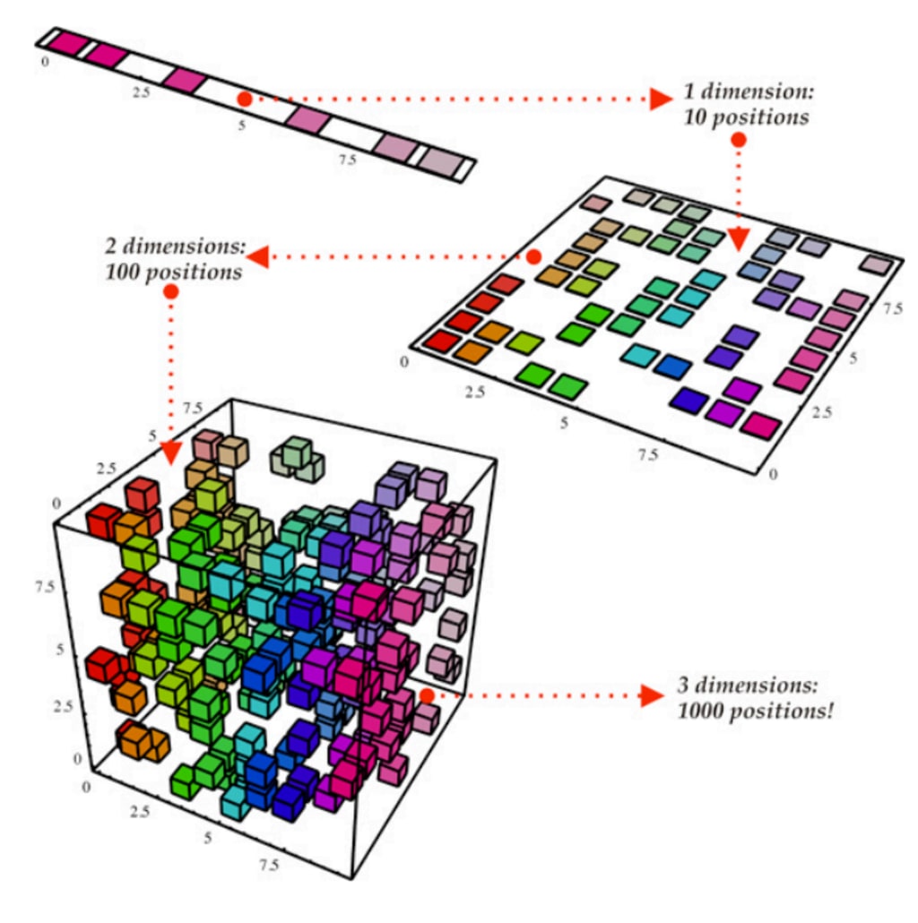
- Faster Execution of Algorithms: PCA can contribute to faster execution of algorithms in certain cases. When dealing with high-dimensional data, the computational complexity of many algorithms increases significantly. By reducing the dimensionality of the data through PCA, the number of variables to process and the computational requirements can be reduced. This can lead to faster execution times for subsequent algorithms that operate on the PCA-transformed data.
- Visualization: PCA can facilitate visualization of high-dimensional data. Visualizing data in more than three dimensions becomes challenging, if not impossible, for humans. By projecting the data onto a lower-dimensional space using PCA, typically two or three dimensions, it becomes feasible to visualize and gain insights from the data. PCA provides a way to represent the data in a simplified manner while preserving as much information as possible.
However, it's worth noting that PCA is not always guaranteed to result in these benefits. The usefulness of PCA depends on the specific characteristics of the dataset and the analysis goals. In some cases, PCA may not significantly improve algorithm execution times, or the visual separation achieved by PCA may not be sufficient for meaningful interpretation.
It's important to consider the trade-offs and limitations of PCA as well. The reduced-dimensional representation obtained through PCA may result in some loss of information, and the interpretability of the transformed variables (principal components) may not always align with the original features.
In summary, while PCA has the potential to lead to faster algorithm execution and aid in visualization, its application should be carefully considered based on the specific context and goals of the analysis
The mathematical formulation of PCA:
Data Standardization: Before performing PCA, the data is standardized by subtracting the mean and dividing by the standard deviation of each variable. The standardized value of each data point is calculated as follows:
std(X) = (X - mean(X)) / std(X)
Covariance Matrix Calculation: The covariance matrix C is computed from the standardized data matrix X_std using the formula:
C = (1 / (n - 1)) * X_std^T * X_std where n is the number of observations in the dataset.
Eigenvalue Decomposition: The covariance matrix C is subjected to eigenvalue decomposition, which yields a set of eigenvectors V and eigenvalues λ:
C = V * Λ * V^T where Λ is a diagonal matrix containing the eigenvalues.
Selection of Principal Components: The eigenvectors V represent the principal components (PCs), where each column of V corresponds to a principal component. The PCs are ranked based on the magnitude of their corresponding eigenvalues. The eigenvectors corresponding to the largest eigenvalues capture the most significant variation in the data.
Dimensionality Reduction: To obtain a lower-dimensional representation of the data, a subset of the principal components is chosen. By selecting k principal components with the highest eigenvalues, the data is projected onto the subspace spanned by these components:
new_X = X_std * V[:, :k]
Here, new_X represents the transformed data matrix in the lower-dimensional space, and V[:, :k] contains the eigenvectors corresponding to the selected principal components.
These mathematical steps outline the core calculations involved in PCA, from data standardization to dimensionality reduction. Implementing these equations allows for the practical application of PCA on a given dataset.
what is matrix transformation?
what are Eigenvalues and Eigenvectors?
Matrix transformation refers to the process of applying a mathematical operation or rule to a matrix, resulting in a new transformed matrix. The transformation can involve operations such as rotation, scaling, reflection, or projection, which modify the original matrix's properties or representation.
Eigenvalues and eigenvectors are important concepts in linear algebra and play a crucial role in various mathematical and scientific applications. They are associated with square matrices, where an eigenvalue represents a scalar and an eigenvector represents a non-zero vector.
Let's delve into more details about eigenvalues and eigenvectors:
Eigenvalues: For a given square matrix A, an eigenvalue (λ) is a scalar that satisfies the equation:
Av=λv
Here, v represents the eigenvector associated with the eigenvalue λ.
In simpler terms, when a matrix is multiplied by its corresponding eigenvector, the result is a scaled version of the eigenvector. The eigenvalue λ determines the scaling factor.
Eigenvalues are important as they provide insights into the matrix's properties, such as its behavior under transformation or its stability characteristics. They are also used in various matrix operations, including matrix diagonalization, matrix exponentiation, and solving systems of linear equations.
Eigenvectors: An eigenvector (v) is a non-zero vector that satisfies the equation:
Av=λv
Here, λ represents the eigenvalue associated with the eigenvector v.
Eigenvectors indicate the directions along which a matrix transformation acts simply by scaling. They describe the fixed directions or subspaces that are unaffected by the matrix transformation, except for scaling. Eigenvectors can be used to understand the behavior and characteristics of the matrix in various applications.
Eigenvectors are not unique and can be multiplied by a scalar factor, while still representing the same direction. Therefore, they are usually normalized to have a unit length, making them easier to interpret and compare.
Eigenvectors are extensively used in applications such as data analysis, image processing, graph theory, and quantum mechanics, among others. They are especially important in techniques like PCA, where they provide the principal components that capture the most significant variations in the data.
In summary, eigenvalues and eigenvectors are fundamental concepts in linear algebra. Eigenvalues represent scalars associated with square matrices, while eigenvectors represent non-zero vectors corresponding to those eigenvalues. They play a crucial role in understanding matrix transformations, stability analysis, and solving systems of linear equations. Additionally, eigenvectors are used in various applications to describe important directions or subspaces in the data or mathematical models.
About the Creator
Keep reading
More stories from ajay mehta and writers in Education and other communities.
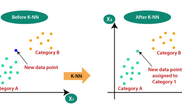
"Unraveling the Power of K-Nearest Neighbors: A Comprehensive Guide to the KNN Algorithm"
K-Nearest Neighbors (KNN) K-Nearest Neighbors (KNN) is a simple, yet powerful machine learning algorithm used for both classification and regression tasks. It makes predictions based on the similarity of input data to its neighboring data points.
By ajay mehta3 years ago in Education
I asked Gemini, Claude, and ChatGPT to create a website, and there was one obvious winner
Vibe-coding seems to be on the rise, and it is fast democratizing software and web development. Not too long ago, a huge barrier of syntax errors separated the average user from developing a website that worked. Times have changed over the last few years. The latest generation of LLMs are powerful and capable enough to turn plain language descriptions into functional code, allowing even non-coders like myself to put together HTML pages with nothing more than a prompt
By Rosalina Jane5 days ago in Education
Governance Leadership in Finance: Strengthening Trust and Driving Competitive Advantage
Governance leadership plays a central role in shaping the stability and credibility of the financial sector. Financial institutions operate in an environment where trust is essential, and strong governance ensures that organizations maintain ethical standards, accountability, and transparency. When governance leaders set clear expectations and enforce responsible practices, they create a foundation that supports both investor confidence and long-term growth.
By Jason Barakat4 days ago in Education


Comments (1)
practical implementation https://www.kaggle.com/nitsin/pca-demo-1 https://github.com/campusx-official/100-days-of-machine-learning/blob/main/day47-pca/pca_step_by_step%20(1).ipynb