
"Unraveling the Power of K-Nearest Neighbors: A Comprehensive Guide to the KNN Algorithm"
Unraveling the Power of K-Nearest Neighbors: A Comprehensive Guide to the KNN Algorithm
K-Nearest Neighbors (KNN)
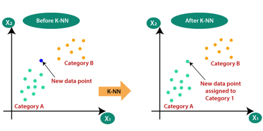
K-Nearest Neighbors (KNN) is a simple, yet powerful machine learning algorithm used for both classification and regression tasks. It makes predictions based on the similarity of input data to its neighboring data points.
Intuition: The intuition behind KNN is that similar data points tend to exist in close proximity to each other. KNN measures the distance between a new data point and existing data points to determine its classification or regression value.
Let's take an example to illustrate this. Suppose we have a dataset with three features: CGPA (Grade Point Average), IQ (Intelligence Quotient), and Placement status (0 for not placed, 1 for placed). We want to predict the placement status for a new student based on their CGPA and IQ.
Let's assume we have the following data points in our dataset:
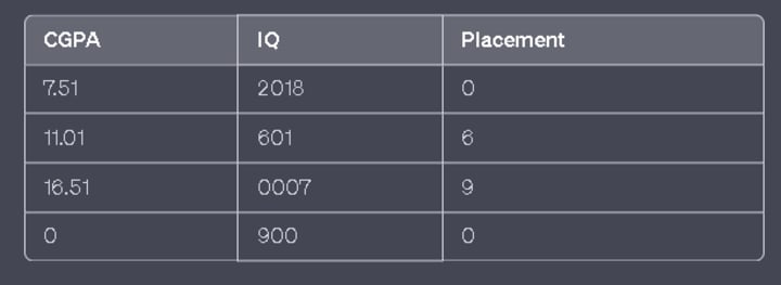
Now, let's say we have a new student with CGPA 7.2 and IQ 105, and we want to predict their placement status using KNN.
- Determine the value of 'K': K represents the number of nearest neighbors we consider when making predictions. Let's say we choose K = 3.
- Measure distances: Calculate the distance between the new student and all the existing data points in the dataset. Common distance metrics include Euclidean distance, Manhattan distance, or Minkowski distance. Let's assume we use Euclidean distance.
- Distance between the new student (7.2, 105) and the existing data points:
- Distance to (7.5, 120) = sqrt((7.5–7.2)² + (120–105)²) ≈ 15.13
- Distance to (8.0, 110) = sqrt((8.0–7.2)² + (110–105)²) ≈ 8.06
- Distance to (6.5, 100) = sqrt((6.5–7.2)² + (100–105)²) ≈ 5.83
- Distance to (7.0, 90) = sqrt((7.0–7.2)² + (90–105)²) ≈ 15.13
- Select the nearest neighbors: Sort the distances in ascending order and select the K nearest neighbors. In this case, we choose the three data points with the shortest distances: (6.5, 100), (8.0, 110), and (7.0, 90).
- Classify or regress: For classification, we assign the most frequent class among the K nearest neighbors to the new student. In this example, if two of the neighbors are placed and one is not, we predict that the new student will be placed. For regression, we take the average or weighted average of the target values of the K nearest neighbors and assign it to the new student.
Data Scaling: If the data is not in the same scale, it can lead to misleading results when calculating distances. Features with larger values will dominate the distance calculations compared to features with smaller values.
To handle this, it's common practice to scale the features to the same range, such as normalization (e.g., min-max scaling) or standardization (e.g., z-score scaling). Scaling ensures that all features contribute equally to the distance calculations, preventing bias towards a particular feature.
By scaling the data, we make sure that the range of values for each feature is similar, allowing KNN to effectively measure distances and find the nearest neighbors based on all features collectively rather than just one dominant feature.
In summary, KNN is an algorithm that makes predictions based on the similarity between a new data point and its nearest neighbors. Scaling the data ensures that all features contribute equally to the distance calculations, avoiding biased results.
Here is the practical implementation of KNN.
knn-on-breast-cancer-dataset | Kaggle
Choosing the value of K in KNN is an important decision that can impact the performance of the algorithm. There are a few commonly used approaches to select K:
- Square Root of N: One heuristic approach is to set K as the square root of the number of data points in the training set (K = sqrt(N)). This approach aims to strike a balance between overfitting (low K) and underfitting (high K). However, this is a rule of thumb and may not always provide the optimal value for K.
- Experimental Evaluation: Another approach is to experimentally evaluate different values of K and choose the one that yields the best performance on a validation set or through cross-validation. You can train and evaluate the KNN algorithm for various values of K and select the one that provides the highest accuracy or other performance metrics.
- Domain Knowledge: Depending on the specific problem and domain, you might have prior knowledge or insights that can guide the selection of K. For example, if you know that the decision boundaries in your data are relatively smooth, you might choose a higher K value. Conversely, if you suspect that the decision boundaries are more intricate, a lower K value could be more appropriate.
It's important to note that there is no universally optimal value for K. The optimal choice may vary depending on the dataset and the specific problem you are trying to solve. It's recommended to experiment with different values of K and evaluate the performance to find the most suitable value for your particular scenario.
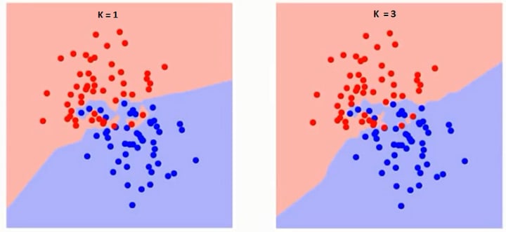
A Decision surfaces.
A decision surface, also known as a decision boundary, is a conceptual boundary that separates different classes or regions in a machine learning model. It helps to visualize how the model distinguishes between different classes based on the input features.
In the case of KNN, the decision surface represents the boundary that determines which class a new data point would belong to based on its nearest neighbors. For example, if we have a binary classification problem with two classes (e.g., "placed" and "not placed"), the decision surface would be the boundary that separates the two classes in the feature space.
To visualize the decision surface of a KNN model, we can use NumPy's meshgrid function. Here's a step-by-step explanation of how it can be done:
- Prepare the data: Consider the dataset with features CGPA, IQ, and Placement. Split the data into features (CGPA and IQ) and the corresponding labels (Placement).
- Train the KNN model: Fit the KNN model using the training data, specifying the desired value of K.
- Create a meshgrid: Generate a grid of points that spans the range of feature values. This is achieved using NumPy's meshgrid function. For example, if we want to visualize the decision surface in a 2D space defined by CGPA and IQ, we create a grid of points covering the range of CGPA and IQ values in the dataset.
- Flatten the grid: Flatten the grid of points to create a list of all coordinate pairs.
- Classify the grid points: Use the trained KNN model to classify each point in the flattened grid by predicting its class based on the nearest neighbors.
- Plot the decision surface: Finally, plot the decision surface using a contour plot or other suitable visualization techniques. Each contour line represents the decision boundary between different classes.
The resulting plot will illustrate how the KNN model separates different classes in the feature space based on the decision surface.
It's important to note that the meshgrid and decision surface visualization can only be done for 2D or 3D feature spaces, as it becomes difficult to visualize higher-dimensional spaces. In higher dimensions, other visualization techniques or dimensionality reduction methods may be used to gain insights into the decision boundaries of the KNN model.
Certainly! Here's an example code snippet in Python using Jupyter Notebook to generate random data points, train a KNN model, and visualize the decision surface using meshgrid and contour:
import numpy as np
import matplotlib.pyplot as plt
from sklearn.neighbors import KNeighborsClassifier
# Generate random data points
np.random.seed(0)
n_samples = 200
cgpa = np.random.uniform(low=6.0, high=9.0, size=n_samples)
iq = np.random.uniform(low=80, high=140, size=n_samples)
placement = np.random.randint(2, size=n_samples)
# Create feature matrix and target labels
X = np.column_stack((cgpa, iq))
y = placement
# Train the KNN model
k = 5 # Value of K
knn = KNeighborsClassifier(n_neighbors=k)
knn.fit(X, y)
# Create a meshgrid
cgpa_range = np.linspace(X[:, 0].min() - 1, X[:, 0].max() + 1, 100)
iq_range = np.linspace(X[:, 1].min() - 1, X[:, 1].max() + 1, 100)
cgpa_grid, iq_grid = np.meshgrid(cgpa_range, iq_range)
grid_points = np.column_stack((cgpa_grid.ravel(), iq_grid.ravel()))
# Classify the grid points
grid_predictions = knn.predict(grid_points)
# Reshape the predictions to match the grid shape
grid_predictions = grid_predictions.reshape(cgpa_grid.shape)
# Plot the decision surface
plt.figure(figsize=(8, 6))
plt.contourf(cgpa_grid, iq_grid, grid_predictions, cmap='coolwarm', alpha=0.8)
plt.scatter(X[:, 0], X[:, 1], c=y, cmap='coolwarm', edgecolors='black')
plt.xlabel('CGPA')
plt.ylabel('IQ')
plt.title('KNN Decision Surface')
plt.colorbar(label='Class')
plt.show()
This code generates random data points for CGPA, IQ, and Placement, trains a KNN model with a chosen value of K (in this case, 5), creates a meshgrid spanning the range of CGPA and IQ values, classifies the grid points using the trained model, and finally visualizes the decision surface using a filled contour plot (contour) overlaid with the scatter plot of the original data points.
You can run this code in a Jupyter Notebook or any other Python environment that supports the required libraries (NumPy, matplotlib, and scikit-learn). Feel free to adjust the parameters and experiment with different values to observe changes in the decision surface.
Overfitting and underfitting are two common issues that can occur when using the K-Nearest Neighbors (KNN) algorithm.
Overfitting:
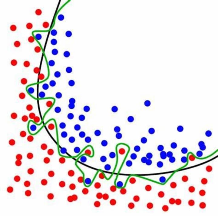
Overfitting happens when the KNN model learns the training data too well and performs poorly on unseen or test data. It occurs when the model becomes too complex, capturing noise or random fluctuations in the training data. In the case of KNN, overfitting can occur when the value of K is too small. This leads to the model being overly sensitive to the training data, resulting in a decision surface that closely fits the training points but fails to generalize well to new data.
To mitigate overfitting in KNN:
- Increase the value of K: By increasing K, the model considers a larger number of neighbors, resulting in a smoother decision surface and reducing the impact of individual noisy data points.
- Regularization techniques: Applying regularization techniques like distance weighting or feature selection can help reduce overfitting in KNN.
- Feature engineering: Preprocess the data by selecting relevant features and removing noise or outliers to improve the model's ability to generalize.
Underfitting
Underfitting: Underfitting occurs when the KNN model is too simple to capture the underlying patterns in the training data. It often happens when the value of K is too large or when the feature space is not adequately represented by the available data. Underfitting leads to high bias, causing the model to have low accuracy both on the training and test data.
To address underfitting in KNN:
- Decrease the value of K: By decreasing K, the model becomes more sensitive to local variations and can capture more complex patterns in the training data.
- Increase the complexity of the model: Consider using more powerful algorithms or techniques that can better capture the underlying patterns in the data.
- Collect more data: Insufficient data might limit the model's ability to learn complex relationships. Obtaining additional data can help improve the model's performance.
- Balancing between overfitting and underfitting involves finding the optimal value of K that generalizes well to unseen data while still capturing the important patterns in the training set. This is often achieved through cross-validation or other model evaluation techniques to select the best value of K.
knn-on-breast-cancer-dataset | Kaggle
Limitations of KNN
K-Nearest Neighbors (KNN) has several limitations that should be taken into consideration when using this algorithm:
- Computationally expensive with large datasets: KNN is a lazy learning algorithm, which means it doesn't learn a model during training. Instead, it stores all training data, making predictions based on the closest neighbors at the time of inference. As a result, the algorithm can be computationally expensive, especially with large datasets, as it requires calculating distances to all training examples.
- Sensitivity to high-dimensional data: In high-dimensional feature spaces, the notion of distance becomes less reliable. This is known as the "curse of dimensionality." As the number of dimensions increases, the points in the feature space become increasingly sparse, and the distance between points tends to become more uniform. This can diminish the effectiveness of KNN in high-dimensional spaces.
- Sensitivity to outliers: KNN is sensitive to outliers as it considers the distances between data points. Outliers can significantly influence the calculation of distances, potentially leading to incorrect classification or regression results. Preprocessing steps like outlier removal or robust distance metrics can be applied to mitigate this issue.
- Non-homogeneous feature scales: KNN relies on distance calculations, and if the features have different scales or units, the feature with larger values can dominate the distance measurements. Therefore, it is important to scale the features before applying KNN to ensure that each feature contributes equally to the distance calculation.
- Imbalanced dataset: KNN can be biased towards the majority class in imbalanced datasets. Since it makes predictions based on the majority of the K nearest neighbors, it may struggle to accurately classify the minority class. Techniques like oversampling, undersampling, or using different distance metrics can help address this problem.
- Lack of interpretability: KNN is not inherently designed for providing interpretable results. It doesn't offer insight into the underlying relationships or feature importance. Additionally, it doesn't provide explicit rules or equations that describe the decision boundaries or decision-making process.
Despite these limitations, KNN can still be a useful algorithm, particularly in cases where interpretability is not a primary concern, and appropriate steps are taken to address its limitations in specific scenarios.
About the Creator
Keep reading
More stories from ajay mehta and writers in Education and other communities.
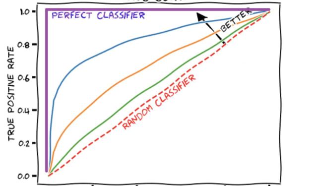
"Mastering ROC AUC Curve: A Comprehensive Guide for Data Scientists"
Why ROC Curve? practical implementation after completing blog. In supervised machine learning, we encounter two types of problems: regression and classification. In a regression problem, we aim to predict a numerical value, such as predicting the salary (LPA) based on features like CGPA and IQ. On the other hand, in a classification problem, we seek to predict the class or category to which a data point belongs. For example, determining whether a student is placed or not based on their CGPA and IQ.
By ajay mehta3 years ago in Education
The Editorial Stack: Building Content Teams for the Multi-Platform Era
In an age where content travels across screens, feeds, formats, and audiences in real time, the old newsroom model no longer fits the demands of digital publishing. Today's media landscape requires more than great writers and sharp editors—it demands a multi-disciplinary, agile, and strategically aligned editorial stack. From video producers to data analysts, newsletter editors to TikTok creators, modern content teams must be designed with versatility and collaboration at their core.
By James Kaminsky18 minutes ago in Education
Hosting a Book Fair
How many of you remember the “best week ever!” from when you were a child? Book fairs were the staple of many of our childhoods with Scholastic leading the way. While there are many choices for book fairs today and I absolutely want to talk about them, that’s going to be a later article.
By Reb Kreyling6 days ago in Education


Comments
There are no comments for this story
Be the first to respond and start the conversation.