Stupid Simple KNN

Summary

In this article you will learn about a very simple yet powerful algorithm called KNN or K-Nearest Neighbor. The first sections will contain a detailed yet clear explanation of this algorithm. At the end of this article you can find an example using KNN (implemented in python).

KNN Explained

KNN is a very popular algorithm, it is one of the top 10 AI algorithms (see Top 10 AI Algorithms). Its popularity springs from the fact that it is very easy to understand and interpret yet many times it's accuracy is comparable or even better than other, more complicated algorithms.

KNN is a supervised algorithm (which means that the training data is labeled, see Supervised and Unsupervised Algorithms), it is non-parametric and lazy (instance based).

Why is lazy? Because it does not explicitly learn the model, but it saves all the training data and uses the whole training set for classification or prediction. This is in contrast to other techniques like SVM, where you can discard all non-support vectors without any problem.

This means that the training process is very fast, it just saves all the values from the data set. The real problem is the huge memory consumption (because we have to store all the data) and time complexity at testing time (since classifying a given observation requires a run down of the whole data set) . But in general it's a very useful algorithm in case of small data sets (or if you have lots of time and memory) or for educational purposes.

Other important assumption is that this algorithm requires that the data is in metric space. This means that we can define metrics for calculation distance between data points. Defining distance metrics can be a real challenge (see Nearest Neighbor Classification and Retrieval). An interesting idea is to find the distance metrics using machine learning (mainly by converting the data to vector space, represent the differences between objects as distances between vectors and learn those differences, but this is another topic, we will talk about this later).

The most used distance metrics are:

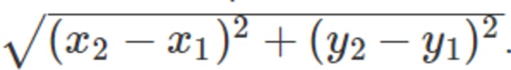
Euclidean Distance:

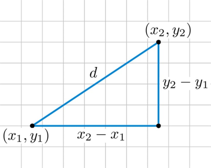
This is the geometrical distance that we are using in our daily life. It's calculated as the square root of the sum of the squared differences between the two point of interest.

The formula is in 2D space:

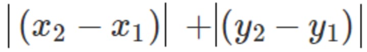
Manhattan Distance:

Calculate the distance between real vectors using the sum of their absolute difference. Also called City Block Distance. You can imagine this as walking in a city which is organized as a matrix (or walking in Manhattan). The streets are the edges of the little squares from the matrix. If you want to go from square A to square B, you have to go on the edges of the little squares. This is longer than the Euclidean distance, because you are not going straight from A to B, but in zigzag.

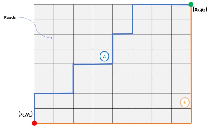
The formula is in 2D space:

Minkowski Distance: Generalization of Euclidean and Manhattan distance. It is a general formula to calculate distances in N dimensions (see Minkowski Distance).

Hamming Distance: Calculate the distance between binary vectors (see Hamming Distance).

KNN for classification

Informally classification means that we have some labeled examples (training data) and for new unlabeled examples (test set) we want to assign labels based on the lessons learned for the training set.

As I said earlier, the KNN algorithm is lazy, there is no learning or generalization in the training phase. The actual work is done at classification or prediction time.

The steps of the KNN algorithm are (formal pseudocode):

1. Initialize selectedi = 0 for all i data points from the training set
2. Select a distance metric (let's say we use Euclidean Distance)
3. For each training set data point i calculate the distancei = distance between the new data point and training point i
4. Choose the K parameter of the algorithm (K = number of neighbors considered), usually it's an odd number, this way avoiding ties in majority voting
5. For j = 1 to K loop through all the training set data points and in each step select the point with minimum distance to the new observation (minimum distancei)
6. For each existing class count how many of the K selected data points are part of that class (voting)
7. Assign to the new observation the class with the maximum count (highest vote) - this is majority voting.

Ok, maybe the formal pseudocode above it's a little bit hard to understand, so let's see the informal explanation.

The main idea is that for a new observation we search the K nearest point (with minimum distance). These points will define the class of the new observation by majority voting.

For example, if we have two classes, red and green and after calculating the distances and getting the 3 nearest points, from which 2 are red and 1 is green, then the selected class by majority voting is red (2 > 1).

If we have to following situation:

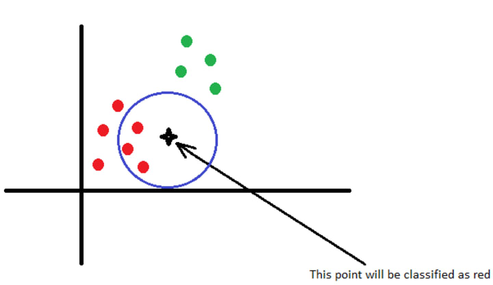
We have two classes, red and green and a new observation, the black star. We choose K = 3, so we will consider the 3 points with minimum distances from the new observation. The star is close to 3 red points, so it is obvious that this new observation will be classified as a red point.

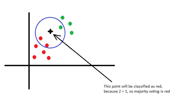
In the picture above I moved the star a little bit closer the the green points. In this case we have 2 red and 1 green points selected. The star will be still classified as red, because 2 > 1.

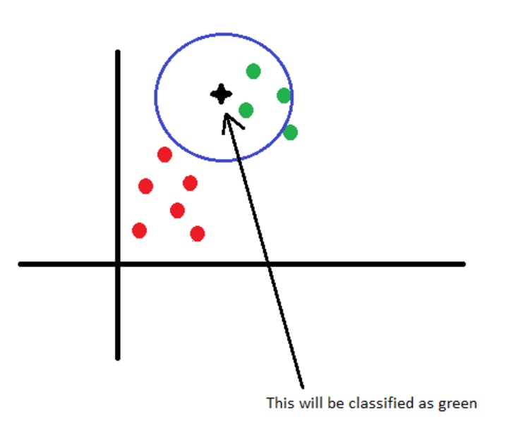
As we move closer to the green points the confidence of selecting red as a label drops, until the new observation will be classified as green. This is the boundary between the red class and the green class, as in the case of different countries. So from a different point of view, we can say that with this algorithm we build the boundaries of the classes. The boundaries are controlled by the value of K. A small K will result sharp boundaries while a big K will result smooth boundaries. The most interesting and most important part is how to choose the best value of K in the context of your specific data set. In the following sections we will see how to choose the best value of K.

What I described above doesn't necessarily mean that the KNN algorithm would always linearly compare the test samples to the training data as if it were a list. The training data can be represented with different structures, like K-D Tree or Ball Tree.

Another improvement is that we can assign weights to the attributes which are more important in the classification. This way, if we know that in our data set there are some important attributes to consider, we can assign them higher weights. This will cause that they will have a greater impact in assigning labels to new observations. The weights can either be uniform (equal dominance of all neighbors) or inversely proportional to the distance of the neighbor from the test sample. You can also devise your own weight assignment algorithm (for example using another AI algorithm to find the most important attributes and assign them higher weights).

KNN for Prediction

Tke KNN algorithm can also be used to predict new values. The most common example is to use KNN to predict the price of something (house, car, etc.) based on the training data. To predict new values, the KNN algorithm is almost the same. In the case of prediction we calculate the K most similar points (metrics for similarity must be defined by the user) and based on these points we can predict new values using formulas like average, weighted average, etc. So the idea is the same, define the metrics to calculate the distance (here similarity), choose the K most similar points and then use a formula to predict the new values based on the selected K points.

Computational Complexity

To calculate the computational complexity of KNN, let's consider a d dimensional space, k is the number of neighbors and n is the total number of training data points.

To understand how can we calculate the complexity of this algorithm, please take a look over the formal pseudocode! Each distance computation requires O(d) runtime, so the third step requires O(nd) work. For each iterate in step five, we perform O(n) work by looping through the training set observations, so the step overall requires O(nk) work. The first step only require O(n) work, so we get a O(nd + kn) runtime. We can reduce this runtime complexity to O(nd) if we use the quickselect algorithm to choose the K points with minimum distances.

How to choose the best K for your data set

You are probably wondering, how can you find the best value for K to maximize the accuracy of the classification or prediction. Firstly I have to mention that the K is a hyperparameter, which means that this parameter is chosen by you, the developer. As I said earlier, you can imagine K as the parameter that controls the decision boundary. For example:

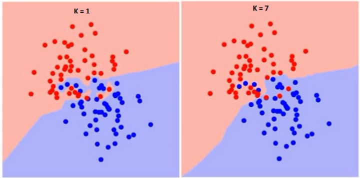
As you can see, if K=1 the border is very sharp, in zigzag but in the case K = 7, the border is smoother. So as we increase the value of K, the boundary becomes smoother. If K would be infinity everything would be blue or red, based on the total majority.

The training error rate and the validation error rate are two parameters that we need to take in consideration when choosing the right K. If the training error is very low but the test error is high, then we have to discuss about overfitting.

Overfitting happens when a model learns the details and noise in the training data to the extent that it negatively impacts the performance of the model on new data. This means that the noise or random fluctuations in the training data is picked up and learned as concepts by the model.

Comparing an overfitted and a regular boundary:

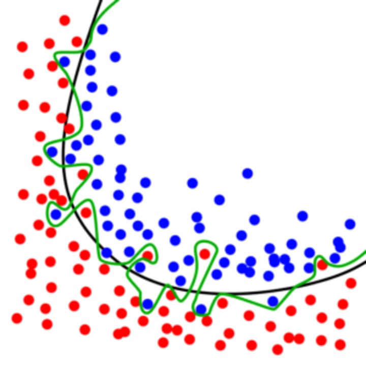
The green line represents an overfitted model and the black line represents a regularized model. While the green line best follows the training data, it is too dependent on that data and it is likely to have a higher error rate on new, unseen data, compared to the black line.

Underfitting refers to a model that can neither model the training data nor generalize to new data. For example using a linear algorithm on non-linear data will have poor performance.

We have to find the golden mean, having a model the can well generalize to new data, but not too well, avoiding to learn the noise and avoiding overfitting.

If we represent the training error rate and the test error rate, we will get some diagrams like the following:

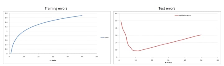
As you can see when K=1 the training error is 0 because the closes point to any training data point is itself. If we look at the test error, when K=1 the error is very high, which is normal because we have overfitting. As we increase the value of K, the test error rate is dropping until it reaches it minimum point, after which the error starts to increase again. So basically the problem to find the best K is an optimization problem, finding the minimum value on a curve. This called the Elbow Method, because the test error curve looks like an elbow.

The conclusion is in order to find the best K use the elbow method and find the minimum on the curve. This can be easily done by brute force, by running the model multiple times, each time increasing the value of K. An efficient way to find the best K is by using K-Fold Cross Validation, but we will talk about this in the last chapter (Boosting the AI Algorithms).

KNN example using Python

In this example we will use the Social_Networks_Ads.csv file which contains information about the users like Gender, Age, Salary. The Purchased column contains the labels for the users. This is a binary classification (we have two classes). If the label is 1 it means that the user has bought product X and 0 means the the users hasn't bought that specific product.

Here you can download the file: Social_Network_Ads.

In this example we will use the following libraries: numpy, pandas, sklearn and motplotlib.

The first step is to import out dataset.

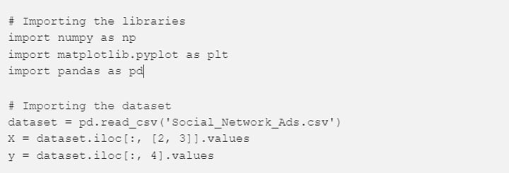
This is an easy task, because the pandas library contains the read_csv method which reads our data and saves it in a data structure called DataFrame.

Most of the algorithms from the sklearn library requires that the attributes and the labels are in separate variables, so we have to parse our data.

In this example (because we want to represent the data in 2-D diagram) we will use only the Age and the Salary to train our model. If you open the file, you can see that the first two columns are the ID and the Gender of the user. We don't want to take these attributes in consideration.

X contains the attributes. Because we don't want to take in consideration the first two columns, we will copy only column 2 and 3 (see line 8).

The labels are in the 4th column, so we will copy this column in variable y (see line 9).

The next step is to split our data in two different chunks, one will be used to train our data and one will be use to test the results of our model (the test attributes will be the new observations and the predicted label will be compared with the labels from the test set).

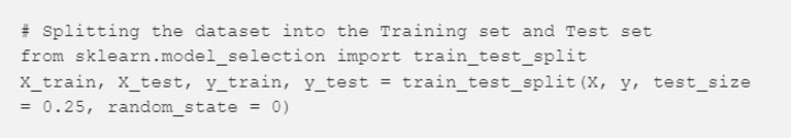
This is another easy task, because sklearn has the method called train_test_split, which will split our data set returning 4 values, the train attributes (X_train), test attributes (X_test), train labels (y_train) and the test labels (y_test). A usual setup is to use 25% of the data set for test and 75% for train. You can use other setup, if you like.

Now take another look over the data set. You can observe that the values from the Salary column are much higher than in the Age column. This can be a problem, because the impact of the Salary column will be much higher. Just think about it, if you have two very close salaries like 10000 and 9000, calculating the distance between them will result in 10000–9000 = 1000. Now if you take the Age column with values like 10 and 9, the difference is 10–9=1, which has lower impact (10 is very small compared to 1000, it's like you have weighted attributes).

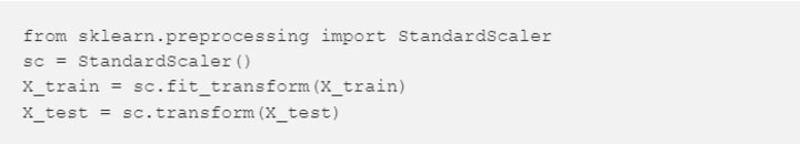
In order to resolve this magnitude problem, we have to scale the attributes. For this we used the StandardScaler from sklearn.

The next step is to train the model:

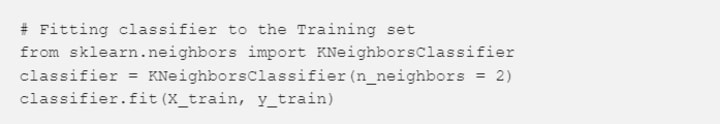
We import the KNeighborsClassifier from sklearn. This takes multiple parameters. The most important parameters are:

1. n_neighbors: the value of k, the number of neighbors considered
2. weights: if you want to use weighted attributes, here you can configure the weights. This takes values like uniform, distance (inverse distance to the new point) or callable which should be defined by the user. The default value is uniform.
3. algorithm: if you want a different representation of the data, here you can use values like ball_tree, kd_tree or brute, default is auto which tries to automatically select the best representation for the current data set.
4. metric: the distance metric (Euclidean, Manhattan, etc), default is Euclidean.

We leave all the default parameters, but for n_neighbors we will use 2 (the default is 5).

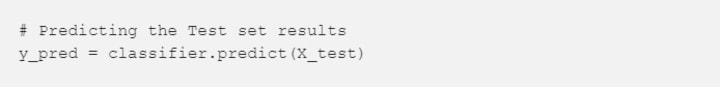
If you want to predict the classes for the new observations, you can use the following code:

The next step is to evaluate our model. For this we will use a Confusion Matrix.

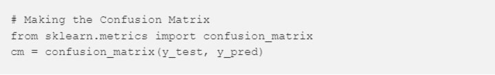
The results of the confusion matrix is:

As you can see we have only 5 False Positives and only 7 False Negatives, which is a really good result (here the accuracy is 80%).

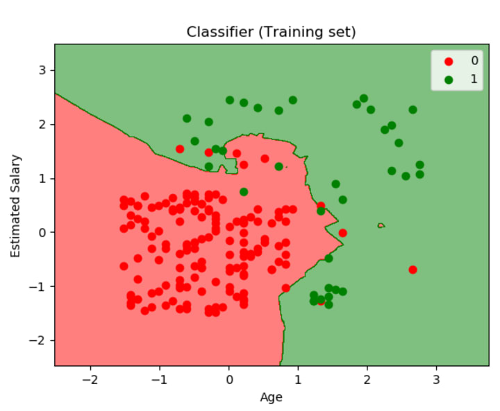
The last step is to visualize the decision boundaries. Let's start with the decision boundaries of the training set.

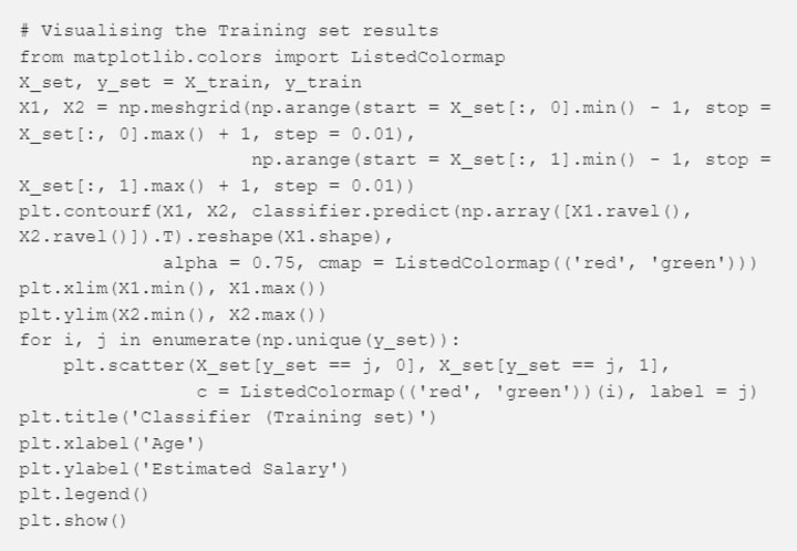
The meshgrid function creates a rectangular grid out of an array of x values and an array of y values (here x = X1 and y = X2).

The contourf method draws filled contours, so we use this method to fill the background with the color of the class associated to it. The trick is that for each pixel we make a prediction and we color that pixel with the color associated to the predicted class. Here we have two classes, we use red and green for 0 and 1.

Between lines 10 and 12 a we loop over all the training data points, we predict the label for them and color them red if the predicted value is 0 and green if the predicted value is 1.

The result of this code is:

To visualize the boundaries of the test set, we use the same code, but changing the X_set, y_set to X_test, y_test. The result of running the code to visualize the boundaries of the test set is:

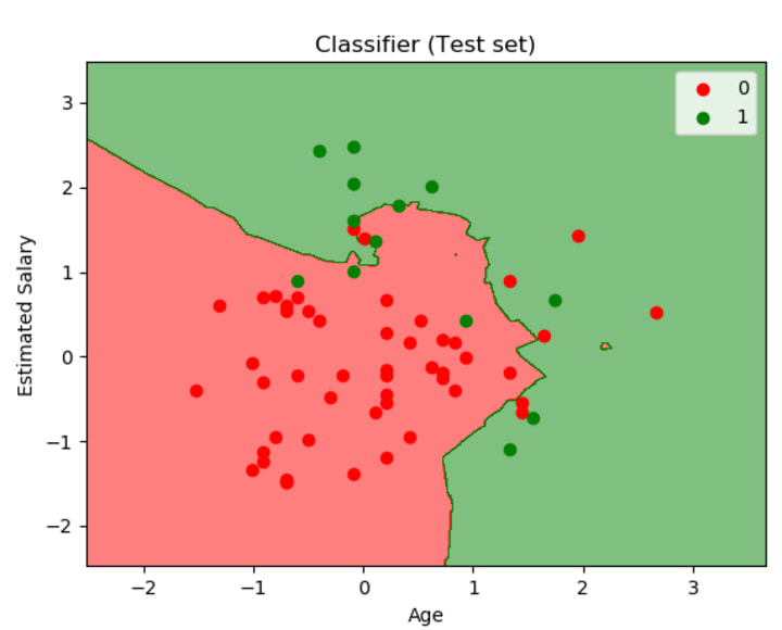
As you can see also in the figure above, we have a really good model, only a few points were wrongly classified.

Conclusions

1. The KNN algorithm is very intuitive and easy to understand
2. The training time is minimal, the model doesn't actually learns or generalizes
3. The testing time can be very long, because the algorithm loops over the whole training dataset and calculates the distances (distance calculation can be a hard work, based on the type of distance metric and based on the type of the dataset)
4. For small K values the algorithm can be noise sensitive and easy to overfit
5. The data set should numeric or a distance metrics should exist to calculate distances between points
6. Doesn't perform too well on unbalanced data.

References

1. Complete Guide to KNN
2. Overfitting and Underfitting in Machine Learning
3. Detailed Introduction to KNN
4. Udemy - Machine Learning from A-to-Z
5. KNN Computational Complexity