Non-Gaussian Probability Distribution

Continuous Non-Gaussian Probability distribution

like uniform distribution, Pareto distribution, log normal distribution

There are also many other non-Gaussian continuous distributions, each with their own applications and characteristics.

2 Discreate Non-Gaussian Probability distribution

What is Uniform Distribution and it's types?

Uniform distribution is a probability distribution where each value in a given interval has an equal probability of occurring. In other words, it is a continuous probability distribution where all values in a given range are equally likely to be observed.

There are two types of uniform distribution:

Continuous Uniform Distribution: In this type of distribution, the values are continuous and can take any value within a given range. For example, the height of a person can be modeled as a continuous uniform distribution between 4 and 7 feet.

Discrete Uniform Distribution: In this type of distribution, the values are discrete and can take only integer values within a given range. For example, the roll of a fair die can be modeled as a discrete uniform distribution between 1 and 6.

Here's an example of a continuous uniform distribution:

Suppose we have a random variable X that represents the time it takes for a customer to complete a survey. We know that the survey takes between 5 and 15 minutes to complete, and any time between 5 and 15 minutes is equally likely. We can model X as a continuous uniform distribution with parameters a=5 and b=15.

The probability density function of the continuous uniform distribution is:

f(x) = 1 / (b-a), for a ≤ x ≤ b = 0, otherwise

The cumulative distribution function of the continuous uniform distribution is:

F(x) = 0, for x < a (x-a)/(b-a), for a ≤ x ≤ b 1, for x > b

The mean and variance of the continuous uniform distribution are:

Mean = (a + b) / 2 Variance = (b - a)² / 12

In our example, the mean of X would be (5+15)/2 = 10 and the variance would be (15–5)²/12 = 8.33.

here are a few more examples of uniform distributions:

A lottery where you choose a number between 1 and 100. Each number has an equal probability of being chosen, so the distribution of winning numbers can be modeled as a discrete uniform distribution.

A random number generator that produces numbers between 0 and 1. If the generator is truly random, the distribution of the numbers produced will be a continuous uniform distribution.

A manufacturing process that produces parts with lengths between 10 cm and 20 cm. If the lengths of the parts are uniformly distributed within this range, we can model the distribution as a continuous uniform distribution.

The arrival time of buses at a bus stop. If the buses arrive at random times between 8:00 AM and 9:00 AM and all times are equally likely, we can model the distribution of arrival times as a continuous uniform distribution.

The weight of a randomly selected apple from a basket of apples. If the apples are all of similar size and weight, we can model the distribution of weights as a continuous uniform distribution between the minimum and maximum weight of the apples in the basket.

USECASE OF UNIFORM DISTRIBUTION

a. Random initialization: In many machine learning algorithms, such as neural networks and k-means clustering, the initial values of the parameters can have a significant impact on the final result. Uniform distribution is often used to randomly initialize the parameters, as it ensures that all values in the range have an equal probability of being selected

a Sampling: Uniform distribution can also be used for sampling. For example, if you have a dataset with an equal number of samples from each class, you can use uniform distribution to randomly select a subset of the data that is representative of all the classes.

b. Data augmentation: In some cases, you may want to artificially increase the size of your dataset by generating new examples that are similar to the original data. Uniform distribution can be used to generate new data points that are within a specified range of the original data.

c. Hyperparameter tuning: Uniform distribution can also be used in hyperparameter tuning, where you need to search for the best combination of hyperparameters for a machine learning model. By defining a uniform prior distribution for each hyperparameter, you can sample from the distribution to explore the hyperparameter space

Log Normal distribution

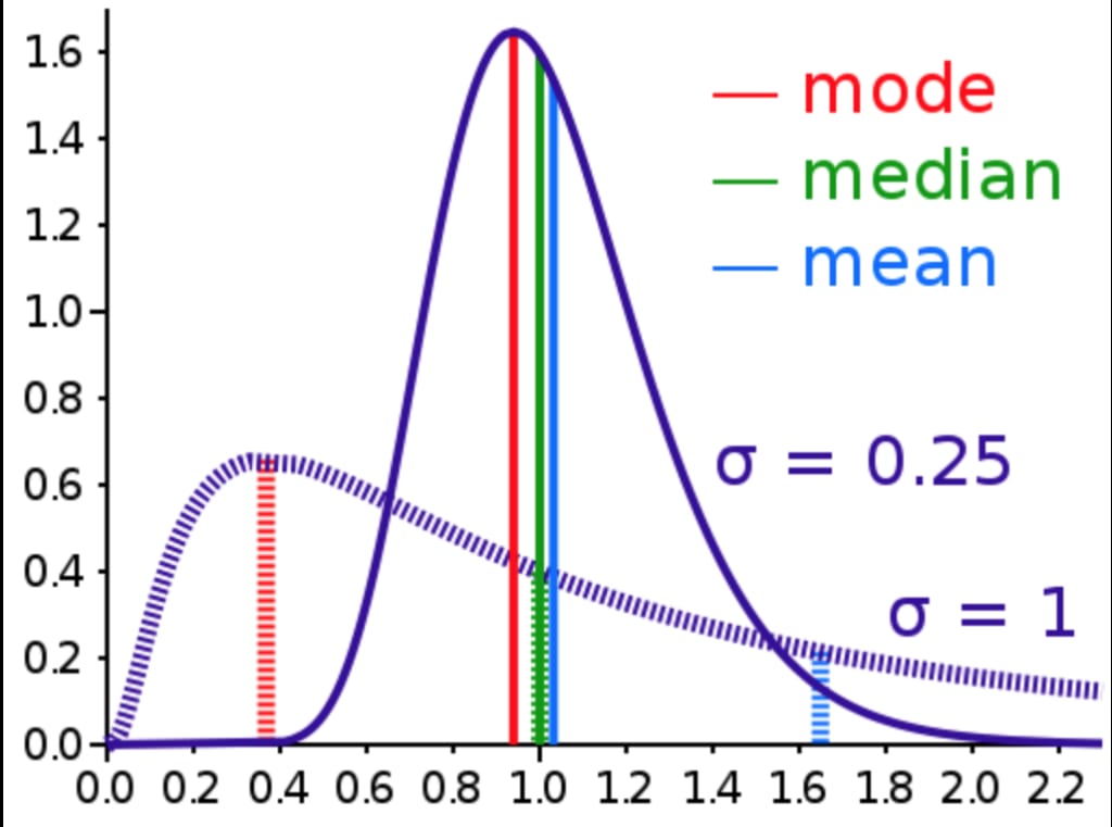
Log-normal distribution is a probability distribution of a random variable whose logarithm follows a normal distribution. In other words, it is a continuous probability distribution of a variable whose natural logarithm has a normal distribution.

In probability theory and statistics, a lognormal distribution is a heavy tailed continuous probability distribution of a random variable whose logarithm is normally distributed

The log-normal distribution is often used to model phenomena that are naturally bounded below by zero, but whose values can vary widely. Examples of such phenomena include the size of populations, incomes, stock prices, and bacterial growth rates.

The probability density function of a log-normal distribution is given by:

f(x) = (1 / (x * σ * √(2π))) * e^(-((ln(x) - μ)² / (2 * σ²)))

where x is the value of the random variable, μ and σ are the mean and standard deviation of the natural logarithm of the random variable, respectively.

Here's an example of how the log-normal distribution can be used in practice:

Suppose we want to model the distribution of the daily returns of a particular stock. We know that the returns are never negative (since the stock price cannot be negative), but can be positive or negative and can vary widely. The log-normal distribution is a natural choice for this application.

We collect historical data on the daily returns of the stock and compute the natural logarithm of the returns. We find that the mean of the logarithms is -0.01 and the standard deviation is 0.03. Using these values, we can compute the parameters of the log-normal distribution as follows:

μ = ln(mean) = ln(e^-0.01) = -0.01005 σ = sqrt(ln(1 + (std² / mean²))) = sqrt(ln(1 + (0.03² / e^-0.01²))) = 0.0317

We can then use the probability density function of the log-normal distribution to estimate the probability of different daily returns. For example, the probability of a return between 1% and 2% can be computed as:

P(0.01 ≤ X ≤ 0.02) = ∫(0.01, 0.02) f(x) dx

where f(x) is the probability density function of the log-normal distribution.

Pareto Distribution

What is Power Law

In mathematics, a power law is a functional relationship between two variables, where one variable is proportional to a power of the other. Specifically, if y and x are two variables related by a power law, then the relationship can be written as: y = k * x^a

Vilfredo Pareto originally used this distribution to describe the allocation of wealth among individuals since it seemed to show rather well the way that a larger portion of the wealth of any society is owned by a smaller percentage of the people in that society. He also used it to describe distribution of income. This idea is sometimes expressed more simply as the Pareto principle or the "80–20 rule" which says that 20% of the population controls 80% of the wealth

The Pareto distribution is a continuous probability distribution used to model phenomena with heavy tails, where a small number of observations account for a large proportion of the total. It is commonly used in economics, finance, and insurance, to model the distribution of incomes, wealth, or losses.

The Pareto distribution has two parameters: the scale parameter (x_m) and the shape parameter (α). The probability density function (PDF) of the Pareto distribution is:

f(x) = α x_m^α / x^(α+1), for x >= x_m

where x is the random variable, x_m is the minimum value of the distribution, and α is the shape parameter.

Here is an example of how the Pareto distribution can be used to model the distribution of incomes:

Suppose we want to model the distribution of incomes in a certain city. We collect a random sample of 1,000 people and ask them their annual income. The data is right-skewed, with a few individuals earning much more than the rest. We suspect that the Pareto distribution may be a good fit for this data.

After analyzing the data, we find that the minimum income in the sample is $10,000, and the average income is $60,000. We estimate the shape parameter of the Pareto distribution to be α=3.5 based on maximum likelihood estimation.

The PDF of the Pareto distribution with these parameters is:

f(x) = 3.5 * 10,000³.5 / x^(3.5+1), for x >= 10,000

We can use this distribution to answer questions such as:

What is the probability that a randomly selected person earns more than $100,000 per year? To calculate this, we need to integrate the PDF of the Pareto distribution from $100,000 to infinity: P(x > 100,000) = ∫f(x)dx = ∫(3.5 * 10,000³.5 / x^(3.5+1))dx from 100,000 to infinity = 0.0116

Therefore, the probability that a randomly selected person earns more than $100,000 per year is approximately 1.16%.

Note that the Pareto distribution is only appropriate for modeling data with heavy tails and a lower bound, such as incomes or wealth. It may not be appropriate for data that do not have a minimum value or have a normal or symmetric distribution.

Transformations

Converting to normal distribution

log transform

reciprocal transformation

power transform (square/square root)

Box cox

yeo Johnson

Function Transformer

Function transformation is a technique used in mathematics and statistics to transform a function from one form to another. The goal of function transformation is to simplify a function or make it easier to analyze, integrate, or differentiate.

Function transformation involves applying a mathematical function to an original function to obtain a new function. The function used to transform the original function is called the transformation function. Some commonly used transformation functions include:

1. Linear transformation: A linear transformation involves multiplying the original function by a constant and adding another constant. This changes the slope and y-intercept of the function but does not change its shape. For example, if we have the function f(x) = x² and we apply a linear transformation by multiplying it by 2 and adding 3, we get the transformed function g(x) = 2x² + 3.
2. Power transformation: A power transformation involves raising the original function to a power. This changes the shape of the function and can make it easier to analyze. For example, if we have the function f(x) = x² and we apply a power transformation by raising it to the power of 1/2, we get the transformed function g(x) = sqrt(x²) = |x|.
3. Exponential transformation: An exponential transformation involves taking the exponential of the original function. This can be useful when dealing with functions that involve exponential growth or decay. For example, if we have the function f(x) = 2x and we apply an exponential transformation by taking e to the power of 2x, we get the transformed function g(x) = e^(2x).
4. Logarithmic transformation: A logarithmic transformation involves taking the logarithm of the original function. This can be useful when dealing with functions that involve multiplication or division. For example, if we have the function f(x) = 2x and we apply a logarithmic transformation by taking the natural logarithm, we get the transformed function g(x) = ln(2x).
5. Function transformation can be a powerful tool in mathematics and statistics. It can be used to simplify complex functions, make them easier to analyze, or make them fit better to certain models or assumptions. However, it is important to carefully choose the appropriate transformation function and to consider any potential drawbacks or limitations of the transformation.